Survey Mode
Survey Mode is designed for GPS-tracked magnetometer surveys — both aerial drone systems and ground-based loggers. It opens by default in Explorer view: your scan overlaid on a live satellite map using your GPS track. From there you can switch to a 2D colour map or a 3D surface model.
Supported instruments
| Instrument | Type |
|---|---|
| PolarWave DroneRover Light | Aerial — entry-level multi-sensor |
| PolarWave DroneRover Professional | Aerial — professional multi-sensor |
| PolarWave DroneRover Enterprise | Aerial — enterprise multi-sensor |
| PolarWave DroneRover Enterprise Max | Aerial — maximum sensor configuration |
| FG Sensors FGA Logger | Ground-based — captures data from up to two fluxgate sensors |
The map overlay requires GPS data embedded in your file. Most FGA Logger exports include this automatically. If the map view is unavailable after upload, verify that GPS was active during your survey. If you are unsure, open the file in a text editor and look for latitude/longitude columns or NMEA sentences near the top.
Uploading a survey file
- Go to Survey under Instruments in the left navigation.
- Click Select File or drag-and-drop your file.
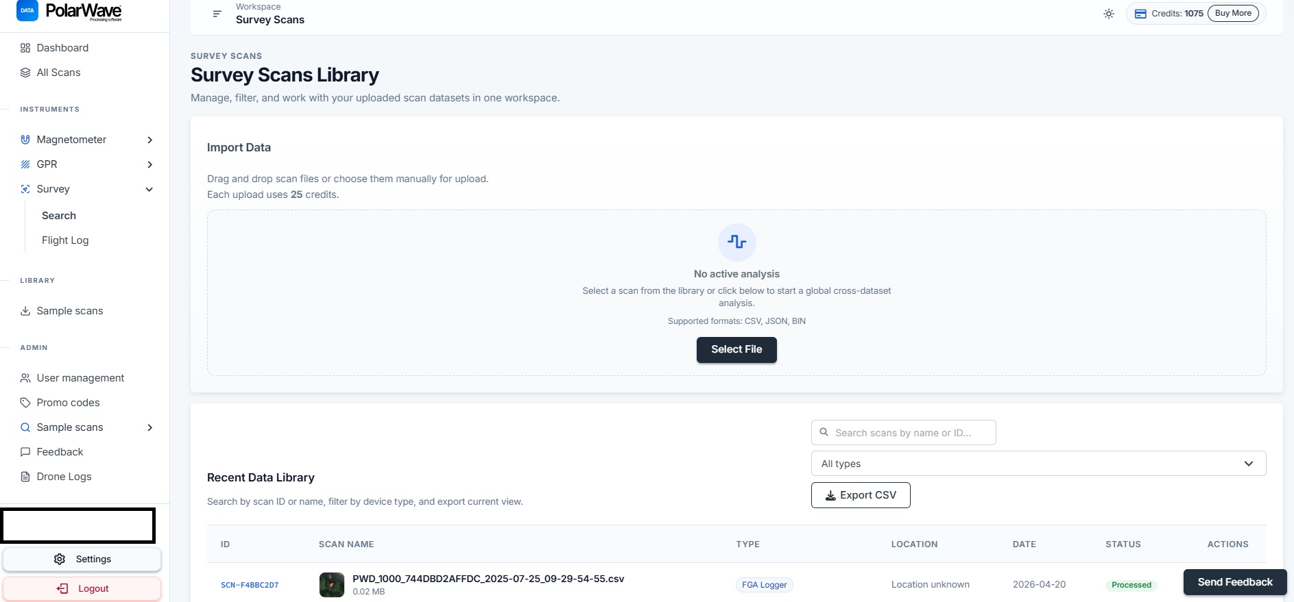
- The platform detects the device type automatically from the filename — keep the original filename intact.
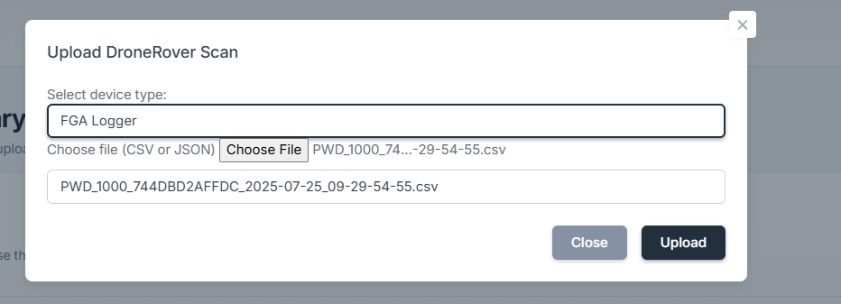
- Click Upload — 25 credits are charged.
- Click the new row to open the map view. Processing typically completes within a few seconds to a minute.

Views
Survey Mode offers three ways to look at your data:
Explorer view (default)
Your scan overlaid on a live satellite map using your GPS track. Individual sensor points are plotted along the flight or survey path. Hover over any point for a tooltip with the channel name and field value.
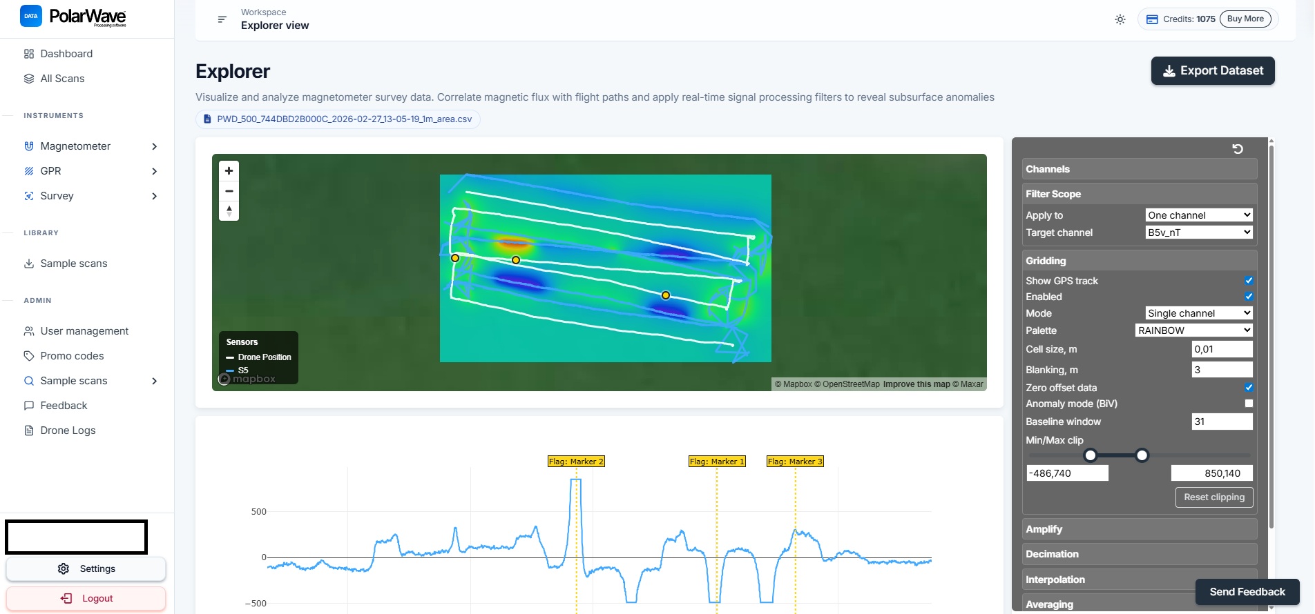
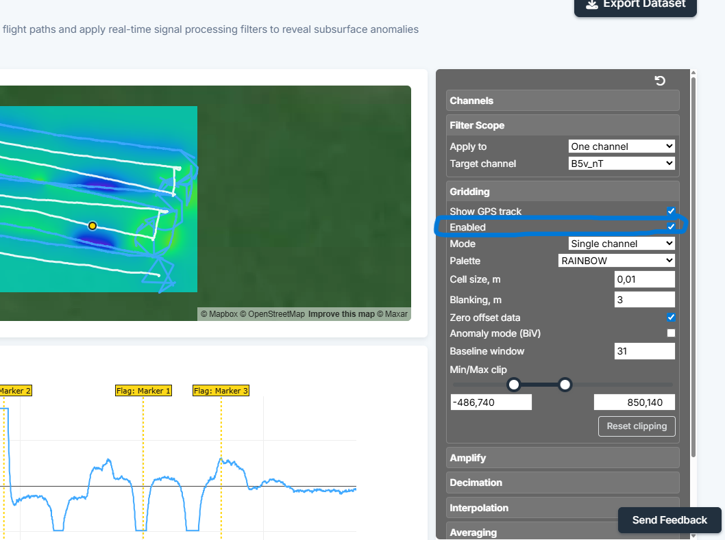
Enable Grid mode to add a colour-coded anomaly overlay directly on the map — all selected sensor readings are interpolated onto a regular grid and rendered over the satellite imagery, so you can see the shape and extent of anomalies in their real geographic context.
If only a GPS track line appears without a colour grid, gridding needs to be switched on in the right-hand panel.
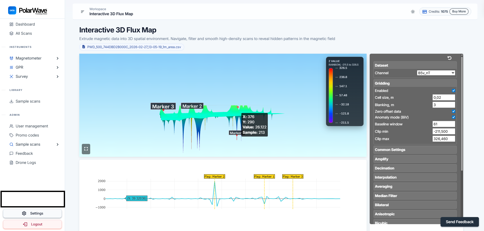
3D surface model
An interactive 3D render showing the depth and shape of anomalies. Peaks and troughs represent measured gradient variations across the surveyed area. Rotate and zoom to inspect the data from any angle.
3D model controls:
| Control | What it does |
|---|---|
| Rotate | Click and drag to spin the model |
| Zoom | Scroll up/down |
| Pan | Right-click and drag (or two-finger trackpad) |
| Tags | Click on the surface to place a marker on a point of interest |
| Vertical exaggeration | Scale the height of peaks and troughs |
Sensor tracks (drone systems)
Each DroneRover sensor records both individual axis readings and a total vector magnitude in nanoTeslas (nT). The channel name encodes the sensor number (B1–B5), the component (x/y/z for individual axes, v for total vector), and the unit (nT).
The number of channels available depends on your DroneRover model — entry-level systems start at two sensors; the Enterprise Max provides all five.
Axis channels (one set per sensor):
| Channel | Description |
|---|---|
| B1x / B2x … B5x | X-axis reading per sensor (nT) |
| B1y / B2y … B5y | Y-axis reading per sensor (nT) |
| B1z / B2z … B5z | Z-axis reading per sensor (nT) |
Vector channels — displayed as colored tracks on the map:
| Channel | Description | Color |
|---|---|---|
| B1v_nT | Sensor 1 — total vector magnitude (nT) | Red |
| B2v_nT | Sensor 2 — total vector magnitude (nT) | Orange |
| B3v_nT | Sensor 3 — total vector magnitude (nT) | Yellow |
| B4v_nT | Sensor 4 — total vector magnitude (nT) | Green |
| B5v_nT | Sensor 5 — total vector magnitude (nT) | Blue |
Toggle individual channels on or off using the legend to isolate a single sensor, or enable All selected to combine them into one grid.
Anomaly grid
When Grid mode is enabled, all selected sensor readings are combined and interpolated onto a color-coded overlay. Large surveys may take a few seconds to render.
FGA Logger channels
The FGA Logger records up to two fluxgate sensors (B1 and B2), each with three axes plus a total vector magnitude. All available channels are listed at the top of the right-hand panel.
| Channel | Description |
|---|---|
| B1x / B1y / B1z | Individual axis readings — sensor 1 |
| B2x / B2y / B2z | Individual axis readings — sensor 2 |
| B1v | Total vector magnitude — sensor 1 (nT) |
| B2v | Total vector magnitude — sensor 2 (nT) |
| Gx / Gy / Gz | Gradient between sensors, per axis (nT/m) |
| Gv | Total gradient vector magnitude (nT/m) |
Click All to show every channel, None to deselect all, or toggle individual channels on and off.
Gv (total gradient) combines all three axes into a single value and is the most sensitive to localised anomalies. Start here for most surveys.
Sensor distance setting
Set the Sensor Distance to the physical separation between your two fluxgate sensors in metres. This value is used to calculate the gradient — an incorrect distance will scale gradient measurements incorrectly.
Map controls
Palette selector
Eleven color palettes are available for the grid overlay:
| Palette | Best used for |
|---|---|
| Thermal | General anomaly detection |
| Viridis | Perceptually uniform, good for publications |
| Rainbow | Maximum color contrast |
| Grayscale | Printing / accessibility |
| Seismic | Bipolar — useful when signal is centered near zero |
| Inferno | High-contrast dark theme |
| Plasma | Vibrant, good on dark backgrounds |
| Magma | Low-light emphasis |
Gridding mode
- Single channel — shows one sensor at a time, useful for comparing sensors individually
- All selected — combines all visible sensors into a single grid
Gaussian normalization
Redistributes the color scale so subtle anomalies are visible even when a single strong feature would otherwise dominate the display.
Sample shift
Applies a time-alignment offset to individual sensors. Use this to correct for small position offsets between sensor tracks that don't correspond to real anomalies.
Reading the map
- Zoom in to an area of interest to see individual sensor track points. Hover over a point for a tooltip with the channel name and field value.
- Enable Grid to see the interpolated anomaly overlay.
- Change the palette if anomalies are not clearly visible — try Thermal or Seismic first.
- Enable Gaussian normalization if one strong anomaly is washing out the rest of the map.
- Toggle sensors on/off using the legend to isolate individual channels.
Live flight mode
When a drone is actively flying and streaming data through the PolarWave mobile app, the mission appears under Live Flights and updates in real time. After landing, the completed mission moves to Survey Scans as a regular scan.
Troubleshooting
| Problem | Likely cause | Fix |
|---|---|---|
| Map shows only a GPS track, no colour grid | Gridding is disabled | Enable the Gridding toggle in the right-hand panel |
| Device type not detected | Filename was renamed | Use the dropdown to select the correct device manually |
| No GPS track visible | GPS was not active during the survey | Re-survey with GPS enabled; verify by opening the file in a text editor and looking for lat/lon columns |
| Gradient values look wrong | Incorrect sensor distance | Set the correct physical sensor separation in metres in the Sensor Distance field |
| Upload fails | File too large or unsupported format | Check that the file is an unmodified FGA Logger export |
Best practices for aerial surveys
- Fly parallel lines at consistent altitude and line spacing (1–3 m depending on target depth).
- Maintain constant speed for even data distribution along each line.
- Keep the sensor altitude as low as safely possible — magnetic signal strength falls off rapidly with distance.
- For multi-sensor systems, verify sensor offset calibration before the survey — incorrect values shift track positions and distort the grid.
- Use Sample Shift if sensor tracks show lateral offsets that don't correspond to real anomalies.