Magnetometer Viewer
The magnetometer viewer is the core analysis tool for TreasureHunter3D and FG Sensors DIY Gradiometer Kit files. After opening a scan you can switch between four view modes using the toolbar at the top of the page.
Uploading a scan
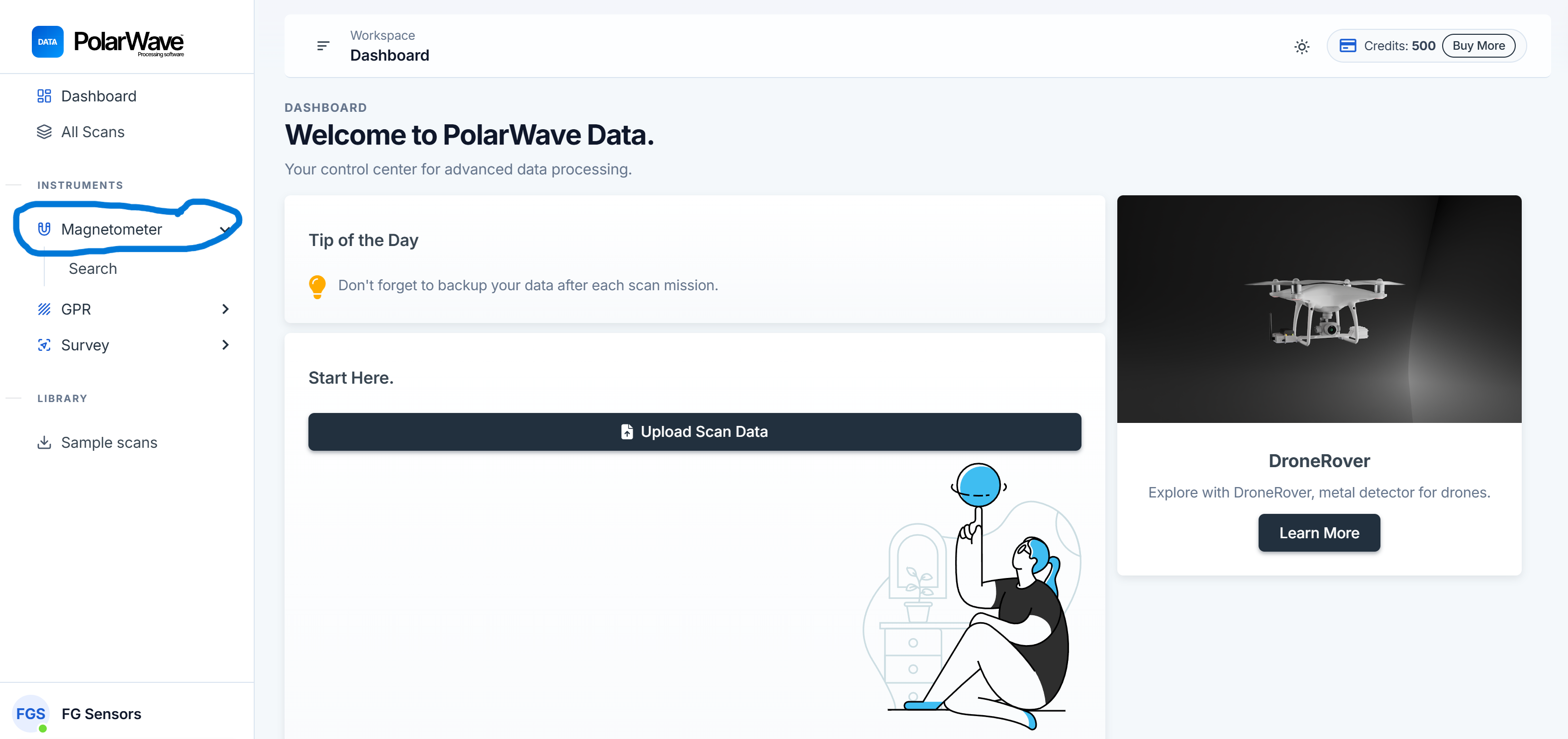
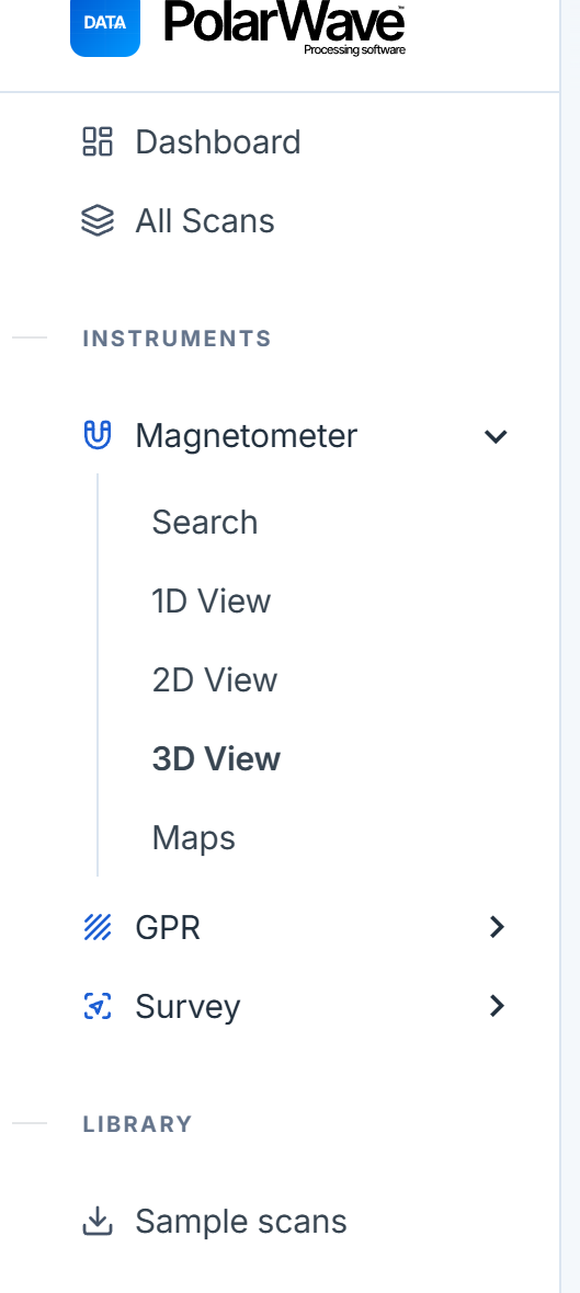
- Go to Magnetometer under Instruments in the left navigation.
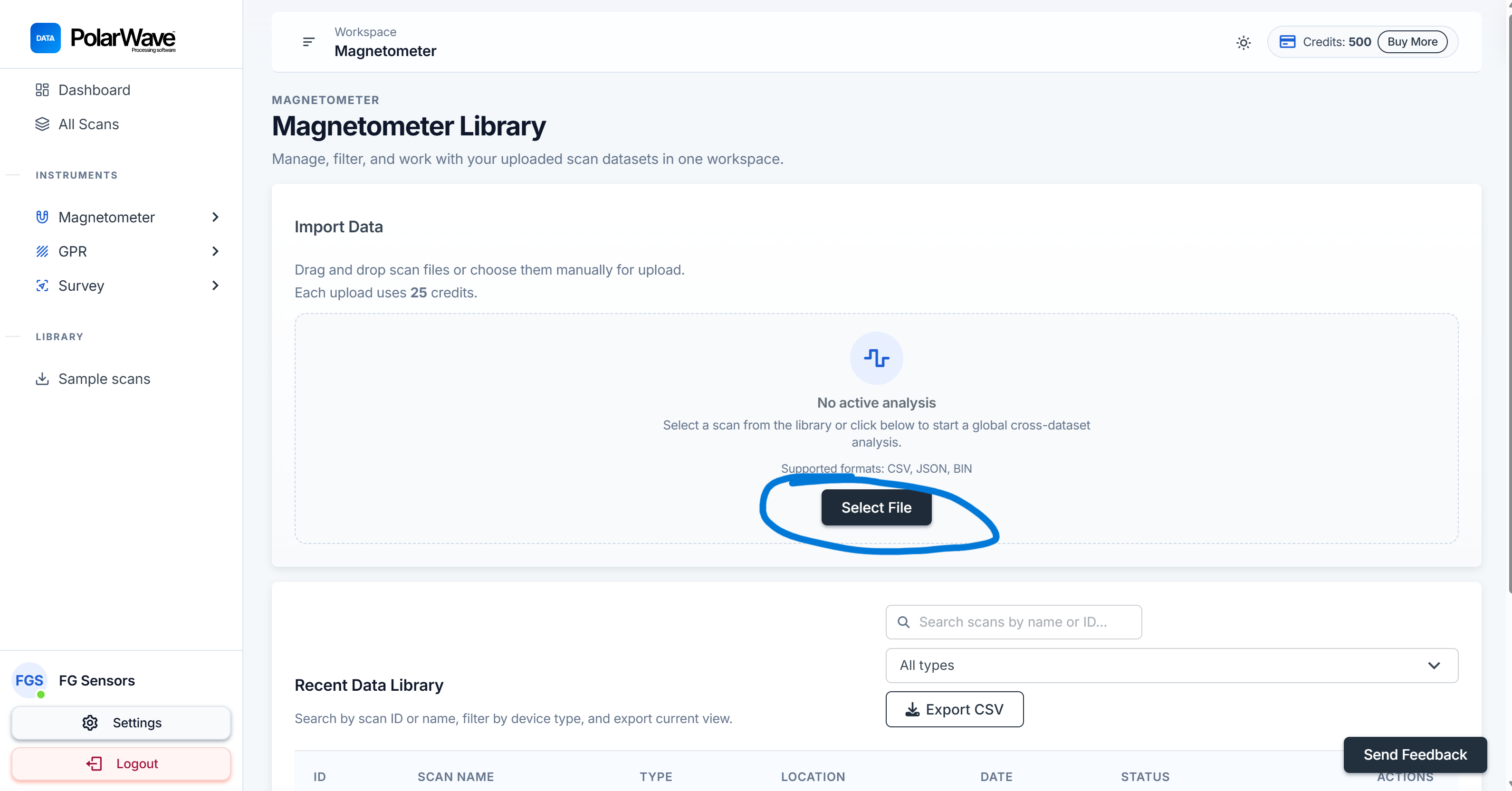
- Click Select File or drag-and-drop your file onto the scan table.
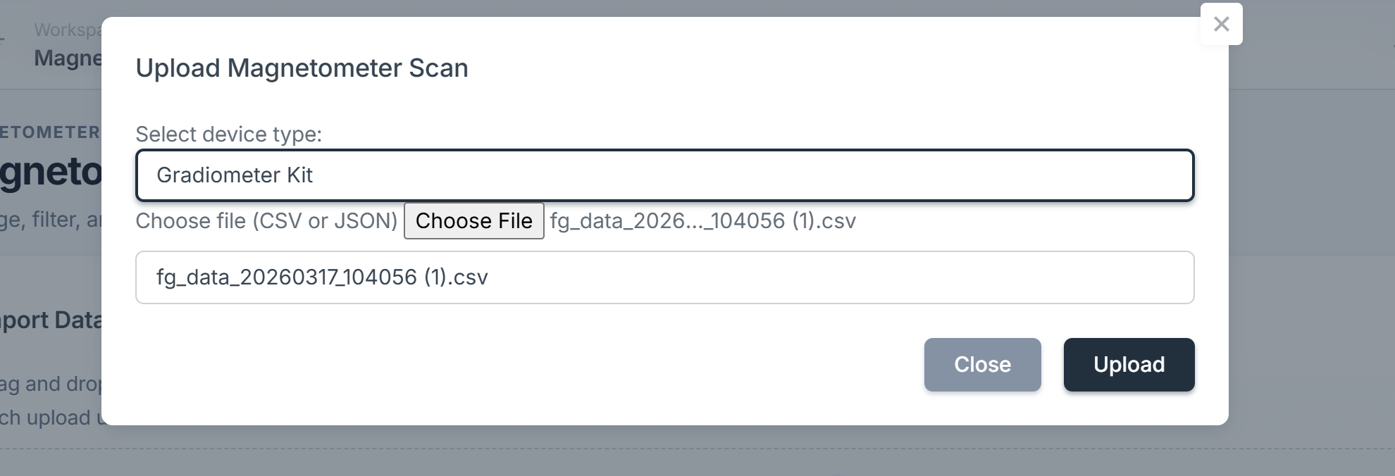
- Choose your device type from the dropdown, or leave it unset for automatic detection. Keep the original filename intact — the platform uses it to identify the device.
- Click Upload — 25 credits are charged. The scan appears in the table within a few seconds to a minute.
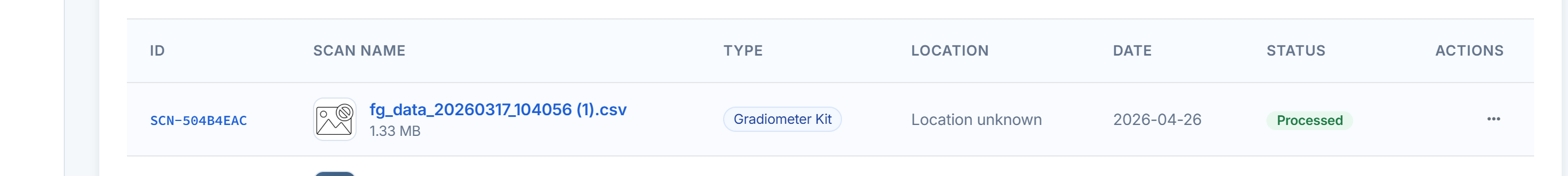
- Click the row to open the viewer. It opens in 3D mode by default, with the 1D profile chart below.
View modes
1D — Profile chart
The 1D view shows your scan as a line graph. The horizontal axis represents position along the scan path and the vertical axis shows signal intensity. The unit depends on your device:
| Device | Unit |
|---|---|
| TreasureHunter3D | Signal strength (–1 to 1) |
| FG Sensors DIY Gradiometer Kit | Signal strength (–1 to 1) |
| PolarWave DroneRover (Survey) | nanoTeslas (nT) |
| FG Sensors FGA Logger (Survey) | nanoTeslas (nT) |
Click on the 1D graph to place a tag on a point of interest — tags are saved with the scan and appear in your PDF report.
Use the mouse wheel to zoom, click-and-drag to pan. Double-click to reset the view.
Controls in the 1D view:
| Control | What it does |
|---|---|
| Magnet Type | Select single-axis, dual-axis, or total field display |
| Metrics Type | Choose the measurement to display (total field, gradient, etc.) |
| Decimation | Thin out the data for faster display of large files |
| Interpolation | Even out the data to a consistent resolution |
| Amplification | Scale up values to make subtle anomalies more visible |
| Smoothing | Reduce noise to reveal the underlying signal shape |
| Detrend | Remove slow baseline drift across the scan |
| Baseline Removal | Center the signal around zero |
| Sensitivity | Adjust the color scale range in 2D and 3D views |
2D — Heatmap
The 2D view renders your scan as a color-coded grid. Rows represent individual scan lines and color represents signal intensity. The same filter controls apply here. Use the Sensitivity slider to bring weak anomalies into the visible range.
Annotations in 2D:
- Click and drag on the grid to draw a rectangular region over an anomaly.
- A dialog will appear asking you to name the region.
- Annotations are saved automatically and appear in your PDF report.
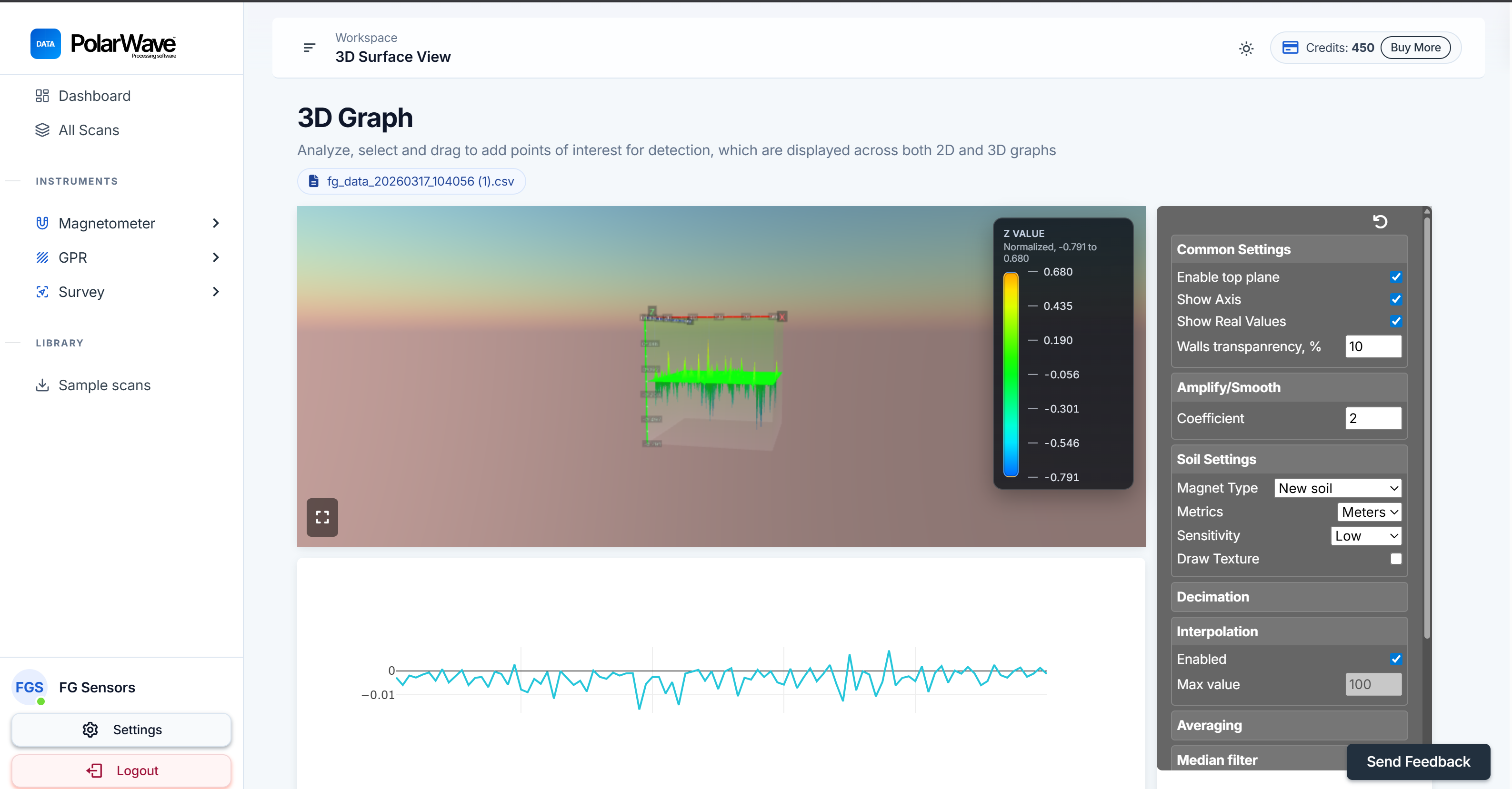
3D — Surface plot
The viewer opens in 3D mode by default. The 3D view renders your data as an interactive three-dimensional surface showing anomaly depth and shape — peaks and troughs represent magnetic field variations across the scanned area.
| Control | What it does |
|---|---|
| Rotate | Click and drag to spin the model from any angle |
| Zoom | Scroll up/down |
| Pan | Right-click and drag (or two-finger trackpad) |
| Tags | Click on the surface to place a marker on a point of interest |
Maps — Satellite overlay
The Maps view displays your scan overlaid on a live satellite or street map using the GPS coordinates recorded during the survey.
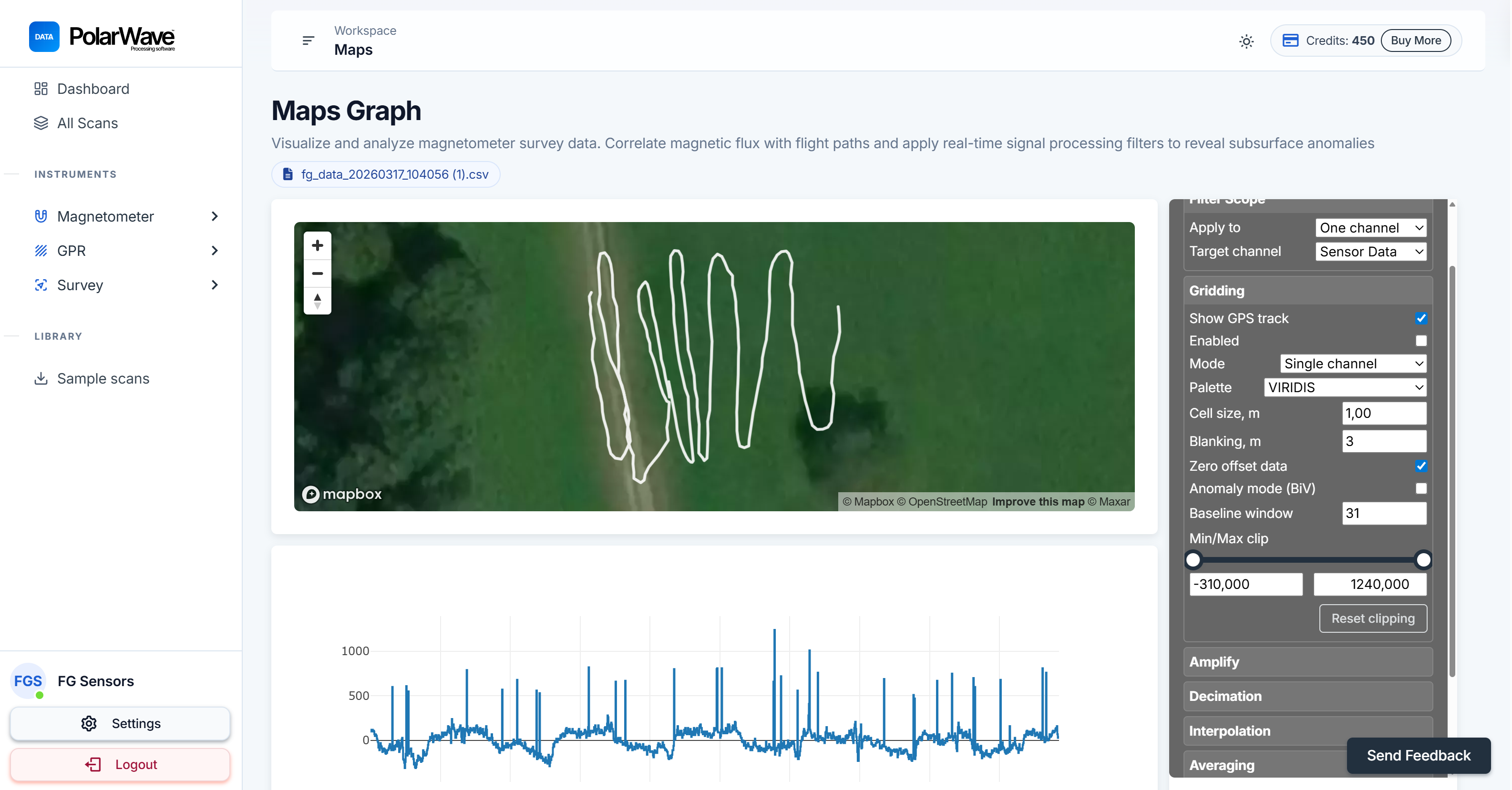
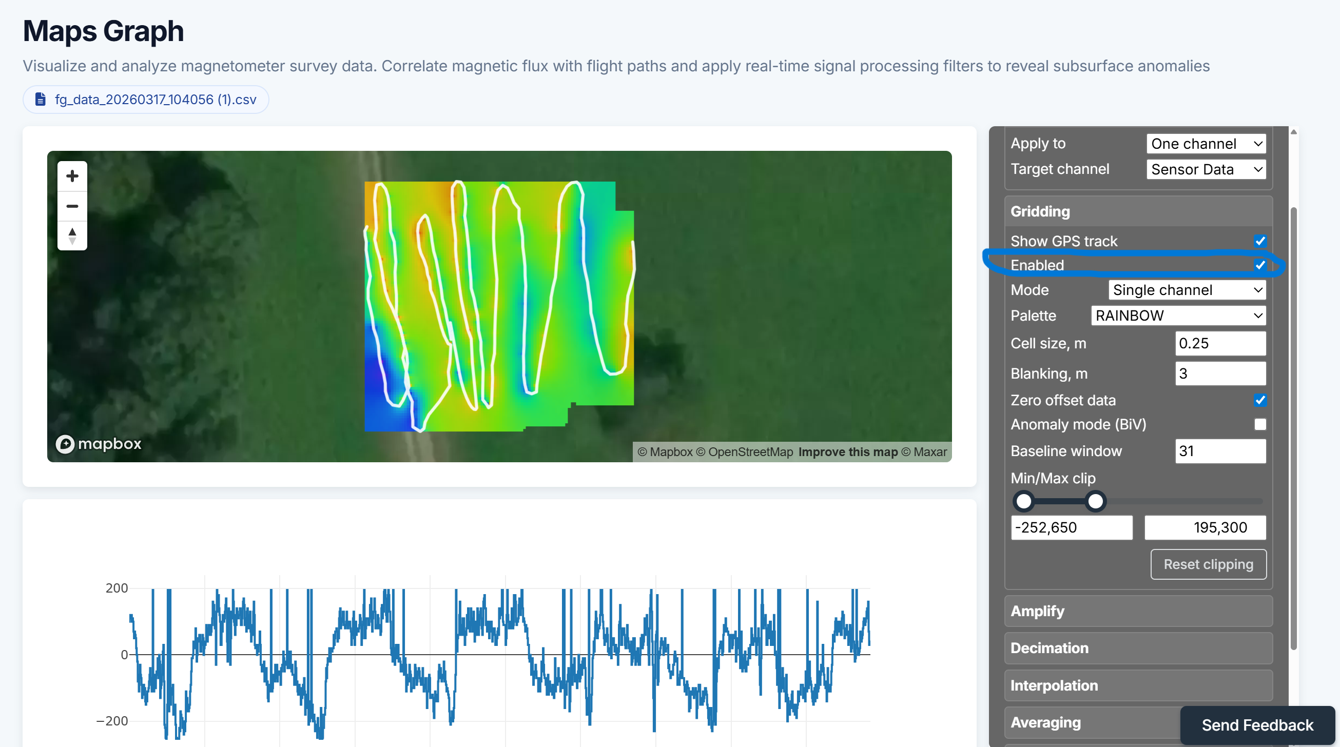
When you first switch to Maps view, a GPS track line appears. Enable Gridding in the right-hand panel to interpolate your survey data across the surveyed area, turning the raw track into a filled colour map.
The Maps view requires GPS data embedded in your file. Confirm GPS logging was active during your survey. If you are unsure, open the file in a text editor and look for latitude/longitude columns near the top.
Patchy or blank areas in the grid usually mean survey lines were spaced too far apart — tighter line spacing produces a smoother, more complete grid.
Toolbar
| Button | Action |
|---|---|
| 1D / 2D / 3D / Maps | Switch view mode |
| Report | Open the report preview for this scan |
| Download CSV | Export the processed data |
Working with multi-axis devices
Devices with 2 or 3 magnetometer axes produce separate channels for each direction. Use the Magnet Type selector to switch between:
- Single axis — vertical component only
- Dual axis — horizontal and vertical
- Total field — combined field strength from all axes
The total-field view is usually the most useful for locating buried ferrous objects.
Tips for finding anomalies
- Apply Detrend first — regional geomagnetic gradients create slow baseline drift that can hide local anomalies.
- Increase Amplification until anomalies stand out from the background.
- Use Smoothing to reduce noise if the signal is very erratic.
- Switch to 2D to see the spatial extent of an anomaly across multiple scan lines.
- Use the Maps view to locate anomalies geographically — enable Gridding for a filled colour overlay.
- Use Tags and Annotations to mark anomaly positions before generating your report.
Filter persistence
All filter settings are saved automatically per scan. When you return to a scan your last configuration is restored. To start fresh, click the Reset Filters button in the filter panel.
Next steps
- GPR Processing →
- Survey Mode →
- Filters & Settings → — Full filter reference
- Generating Reports →